Mike Ravella, Don Lance and Tim Allen
Department of Geology, Mailstop 2001
Keene State College, Keene, NH 03435-2001
August 1996
Mike Ravella, Don Lance and
Tim Allen
Department of Geology, Mailstop 2001
Keene State College, Keene, NH 03435-2001
August 1996
We determined soil infiltration rates and soil moisture contents, and monitored soil tension, water table and piezometric head levels over time at selected sites, in an effort to develop a better understanding of ground water recharge processes and to identify aquifer recharge areas in the Keene region.
The project was conducted as an Independent Study by Ravella and Lance under the direction of Professor Tim Allen, part of on-going work on Ground Water Recharge and the Hydrogeology of Keene. As an introduction, one might read Ravella and Lance's successful Proposal to the Keene State College Undergraduate Research Fund.
The hydrologic cycle is a complex process continually recycling water here on earth (Figure 1a). An important reservoir of water in the hydrologic cycle is that of ground water, which receives recharge primarily from the infiltration of precipitation that falls on the earth's surface. In order to recharge ground water aquifers, this infiltrating water must pass through the vadose or unsaturated zone (Figure 1b). The water in this zone only partially fills the pore spaces between the mineral and organic grains of the soil and is under tension because it is held tightly between these particles by forces of adhesion and cohesion (Sanders, 1996). Below, in the phreatic or saturated zone (Figure 1b), water completely fills the pore spaces between grains. In between these two zones is an area known as the capillary fringe, where the pore spaces are completely filled with water (saturated) but that water is under tension due to cohesion and adhesion to the grains.
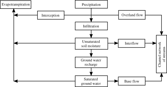
Figure 1a: Schematic diagram of the Hydrologic Cycle (after Domenico &
Schwartz, 1990)
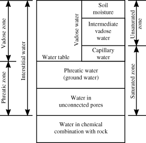
Figure 1b: Subsurface water profile (after Domenico & Schwartz,
1990)
The objective of this project was to study the infiltration of water through the unsaturated (vadose) zone to the saturated (phreatic) zone (Figure 1b), for the purpose of understanding recharge processes, identifying aquifer recharge areas and quantifying recharge rates. We compiled a map of A-horizon soil permeability (Plate 1) in the Keene region (Moore et al., 1994) from data in the USDA Soil Conservation Service Soil Survey for Cheshire County (Rosenberg, 1989). From this map, we selected several sites of both high and low permeability for further study: the College Fields, the College Camp, and the Keene Forestry Park (Figure 2). At each of these sites, we determined soil infiltration rates (Tricker, 1978, 1981) and soil moisture contents and installed tensiometers, wells and piezometers. We then monitored soil tension, water table and piezometric head levels over time (Dingman, 1994). Differences in these levels at each site were used to calculate vertical hydraulic head gradients and determine whether the site was experiencing recharge or discharge (Domenico & Schwartz, 1990). Precipitation data was obtained from the US Army Corps of Engineers at Otter Brook Dam. During this project we have also gained experience in a variety of scientific field measurement techniques, and the analysis and interpretation of data.
Figure 2: Map showing locations of instrumented field sites.
This work is important because ground water is an invaluable but limited resource, providing water for drinking, irrigation and other uses. Understanding recharge processes and quantifying recharge rates enables us to better evaluate ground water resources and determine sustainable yields. Identifying aquifer recharge areas is important, as any pollution in these areas could effect the cleanliness of the aquifers and the purity of the water that comes from them.
One site that we chose for this project was the College Camp, adjacent Wilson Pond in North Swanzey (Figure 2). According to the Soil Survey (Rosenberg, 1989) the soils at this site have an A-horizon permeability of between rate of 6.0 to 20.0 inches/hour (15 to 50 cm/hour). This is a relatively high infiltration rate for Keene-area soils, so this is a potential site for aquifer recharge or local recharge to Wilson Pond. The site is underlain by loam, clay, and sand; soil boring logs for the site are shown in Figure 3. At this location we installed two observation well/piezometer pairs, one 3 meters deep on a lower terrace near Wilson Pond (CC1W & CC1P), the second 4.2 meters deep on a higher terrace further from the pond (CC2W & CC2P). Their relative positions, as well as their relationship to the pond, are shown in cross-section in Figure 12. Dimensions and elevations for all wells and piezometers are given in Table 1. In addition to determining vertical hydraulic gradients at each well/piezometer pair, the set of two well/piezometer pairs was also used for determining horizontal hydraulic gradients. One foot (0.3 meter) and 3 foot (0.9 meter) tensiometers (CCT1 & CCT3) were installed adjacent CC2W & CC2P in order to measure the soil tension at the site and the vertical hydraulic gradient in the unsaturated zone.
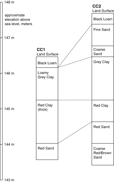
Figure 3: Soil boring logs from the College Camp site
Another of the sites chosen was located in Keene State College's fields south of the athletic stadium off the end of Krif Road, in the flood plain of the meandering Ashuelot River and adjacent to an oxbow lake (Figure 2). We choose this location because it represented a majority of the soils in the Keene region (fine sandy loam). This site is also relatively accessible from campus, and some instrumentation already existed there. According to the Soil Survey (Rosenberg, 1989), the soils at this site have an A-horizon permeability of between 0.6 to 6 inches/hour (1.5 to 15 cm/hour). The water table is relatively shallow.
At this site, there is a City monitoring well tapping a deep aquifer (TW#6). Artesian water levels in this well indicate the deep aquifer is confined, and that the site is within a regional discharge area. Additional instrumentation installed here include a drainage lysimeter (CFLS & CFLD) for monitoring evapotranspiration, a 3 meter deep water table observation well (CF1W), a 3.6 meter deep observation well and piezometer pair (CF2W & CF2P), and 1 foot (0.3 m) and 3 foot (0.9 m) tensiometers (CFT1 & CFT3) with soil thermometers.
The third site that we decided to use was at the Keene Forestry Park, across from the Keene Airport in North Swanzey (Figure 2). This site was chosen because the Soil Survey (Rosenberg, 1989) suggests the soils at this site have an A-horizon permeability rate of greater than 20.0 inches/hour (50 cm/hr). This rate is the highest rate of all the soils in the Keene area (Plate 1). This site has a swamp in its lowlands, and a perched wetland in its highlands, with a (man-made) "disappearing" stream between the two. The site is underlain primarily by sands, although a clay was encountered near the bottom of our borings; soil boring logs for the site are shown in Figure 4. We installed four observation well/piezometer pairs, evenly distributed between the lowland swamp and the upper perched wetland (KFP1W & KFP1P through KFP4W & KFP4P). Their relative positions, as well as their relationship to the pond, are shown in cross-section in Figure 16. In addition to determining vertical hydraulic gradients at each well/piezometer pair, the set of four well/piezometer pairs was also used for determining horizontal hydraulic gradients. No soil tensiometers were installed at this site.
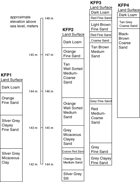
Figure 4: Soil boring logs from the Keene Forestry Park site.
| ID # | MP above local datum | MP above sea level | MP above Ground | Well Depth | Casing Length | Screen Length |
|---|---|---|---|---|---|---|
| College Camp | ||||||
| Pond | 0.00 | 145.00 | ||||
| CC1W | 1.62 | 146.62 | 0.170 | 1.805 | 3.05 | 2.44 |
| CC1P | 1.62 | 146.62 | 0.170 | 2.289 | 3.05 | 0.00 |
| CC2W | 3.05 | 148.05 | 0.380 | 3.277 | 4.42 | 3.51 |
| CC2P | 3.05 | 148.05 | 0.380 | 3.437 | 4.42 | 0.00 |
| CCT1 | 2.19 | 147.19 | -0.3 | |||
| CCT3 | 1.62 | 146.62 | -0.9 | |||
| College Fields | ||||||
| Oxbow | 138.7-140.0 | |||||
| Storage Pond | 139.6-140.1 | |||||
| CF1W | -0.37 | 140.33 | 0.145 | 3.040 | 3.05 | 2.44 |
| CF2W | 0.46 | 141.16 | 0.140 | 2.697 | 3.66 | 3.05 |
| CF2P | 0.46 | 141.16 | 0.140 | 2.935 | 3.66 | 0.00 |
| TW#6 | 0.00 | 140.70 | 0.420 | 49.070 | 44.81 | 3.05 |
| CFT1 | -0.74 | 139.96 | -0.3 | |||
| CFT3 | -1.37 | 139.33 | -0.9 | |||
| Keene Forestry Park | ||||||
| Lower Wetland | 0.00 | 142.00 | ||||
| KFP1P | 2.47 | 144.47 | 0.240 | 1.852 | 3.05 | 0.00 |
| KFP1W | 2.47 | 144.47 | 0.240 | 2.410 | 3.05 | 2.44 |
| KFP2P | 5.97 | 147.97 | 0.470 | 3.945 | 4.57 | 0.00 |
| KFP2W | 5.97 | 147.97 | 0.470 | 3.945 | 4.57 | 3.05 |
| KFP3P | 6.55 | 148.55 | 0.305 | 3.815 | 4.57 | 0.00 |
| KFP3W | 6.55 | 148.55 | 0.305 | 3.835 | 4.57 | 3.05 |
| KFP4P | 6.58 | 148.58 | 0.412 | 2.765 | 3.05 | 0.00 |
| KFP4W | 6.58 | 148.58 | 0.412 | 2.780 | 3.05 | 2.59 |
| Upper Wetland | 5.76 | 147.76 | ||||
Table 1: Dimensions and elevations for wells, piezometers, and tensiometers used in this study. All values in meters. �MP� refers to the Measuring Point on the well or piezometer, usually the top of the casing. The �MP� of the tensiometers is the porous ceramic cups at their tips. References to sea level obtained by map interpolation.
Field work for this study was carried out in the fall of 1995 and the spring of 1996. Infiltration tests were conducted at the College Fields and the College Camp in the fall; and at the College Camp and the Keene Forestry Park in the spring. In the fall, soil tension values and water table elevation at the College Fields site were recorded twice daily (early morning and late afternoon) through the month of October. In the spring, soil tension values, water table elevations, and piezometric head levels at all sites were recorded daily beginning in mid March, through the end of April.
By measuring the infiltration rate of soils we can develop a quantitative understanding of the infiltration process which is a critical component of the hydrologic cycle and ground water recharge. Infiltration capacity is defined as the maximum rate at which a given soil with a given condition can absorb rain as it falls (Tricker, 1981). In our study, however, no simulation of rain fall was made so the measurements are accepted as water penetration instead of rainfall infiltration (Tricker, 1979).
Field measurements for values of infiltration were obtained by use of cylinder infiltrometers (Figures 5 and 6), made from sections of 15 cm diameter plastic sewer pipe. These have proven to be the easiest to make and to operate compared with rainfall simulation devices or larger ring-type infiltrometers. For each measurement site, ten cylinder infiltrometers were spread out over a twenty square meter area (Figure 5), in order to get a representative average at the site. These cylindrical infiltrometers were pushed 5 cm into the ground, and the water within the cylinder was kept at a constant head of 5 cm. We maintained this constant head by suspending a 2 liter soda bottle filled with water at the 5 cm of head mark. The 2 liter bottle had a slanted opening which allowed for air to seep into the bottle when the head got lower then 5 cm. This air caused the water in the bottle to flow out until the head returned to the initial 5 cm height, which then stopped air from going into the bottle and in turn stopped the water from flowing out (Figure 6). We ran our infiltration tests for one hour as Tricker (1981) did. This allowed ample time for the soil to become truly saturated. Running each test for the same amount of time allowed their results to be easily compared. We also kept track of the initial "instantaneous" infiltration rates and the final "instantaneous" infiltration rates, by measuring for 5 minutes at the beginning and end of the hour.
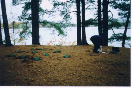
Figure 5: Infiltration Test at the College Camp site, with 10 ring-infiltrometers evenly
distributed over a 20 square meter area.
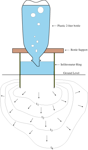
Figure 6: Infiltrometer, showing 2-liter bottle used to maintain constant head, and pattern of
wetting front advancement over time (t1 - t4; after Dingman, 1994).
The measurement recorded in each test was the amount of water required in order to maintain the 5 cm of head within the infiltrometers over the elapsed time. Infiltration rates were calculated in inches per hour from the volume consumed, the cross-sectional area of the cylinders, and the elapsed time.
A problem with the ring infiltrometers is lateral seepage (Figure 6). This is partly due to the fact that the water is infiltrating into unsaturated soil and is influenced by both capillary and gravitational forces. As a result water applied to the infiltrometer ring moves both laterally and vertically (Dingman, 1994). We did not make any attempts to compensate for this, such as double-ring techniques; rather we used the correction factors derived by Tricker (1978).
Another factor to be considered in interpreting infiltration test results is the degree of saturation or soil moisture content at the time of the test.To assess this, we collected soil samples with a sliding-hammer soil-corer at each test site. The corer collects samples 2" in diameter, 6" long (5 cm by 15 cm). These were sealed in plastic bags to preserve their moisture content. In the laboratory, the soil bags were weighed, and then the soil was dryed in a drying oven (105 °F or 40.5 °C) overnight, and weighed again. Soil moisture content was determined by the difference between wet and dry weight. Porosity was determined from the dry weight, sample volume, and an assumed density of 2.65 g/cm3 for the soil solids. Saturation was determined from the difference between wet and dry weight and the calculated pore volume.
The drainage lysimeter, used for monitoring infiltration and evapotranspiration, was installed at the College Fields site in September, 1995. The installation was quite simple. We dug out a hole 1.5 meters square, 1.5 meters deep, to accept the lysimeter box (a steel box 1.5 meters deep, and 1.2 meters by 1.2 meters wide, with a slanted bottom; Figure 7), separating the different layers soil according to the order in which they were removed, on plastic sheets laid out for this purpose. We then placed the lysimeter box in its hole and leveled it. We placed two observation wells in the lysimeter--one in the deep corner and one in the shallow corner, and replaced the soil layers in the same order in which they were removed. We tried to minimize the amount of disturbance so that these soils would be representative of the surrounding area. Despite our efforts to minimize disturbance there was excess soil after installation, due to the fact that soil expands during excavation and we had insufficient compaction when we put the soil back into the lysimeter. The excess soil was mounded over the lysimeter so that as the soil compacted, there would not be a depression. Eventually, the material in the lysimeter will obtain its original properties and give a good representation of the surrounding soil type. Although we did monitor water levels in the lysimeter, no interpretation of that data has yet been made.
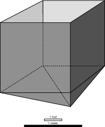
Figure 7: Drainage lysimeter design.
Wells and Piezometers were installed by auguring 3" (7.5 cm) diameter holes with a hand bucket auger (Figure 8), to depths ranging from 2 to 4.5 meters, depending on the level of the water table at each site. While we were auguring the holes we kept a boring log of the different layers of soil that we encountered and what they were composed of. With these boring logs we created soil profiles for each site (Figures 3 and 4). We used 1" (2.5 cm) diameter PVC pipes for both the observation wells and the piezometers (Figure 9). This made it quite convenient because we could fit both of these in the same 3" (7.5 cm) diameter hole, reducing the number of holes that we had to auger by half. The wells used to monitor the water table were slotted with a hacksaw all the way from their bottoms to a height well above the water table. The piezometers were open only at their bottoms, to monitor the hydraulic head at that depth. The relative elevations of the measuring points for each well and piezometer were determined by level surveying at each site (Table 1).
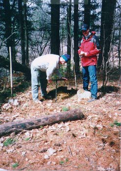
Figure 8: Installing wells and piezometers with a hand auger, logging soils as hole is
bored.
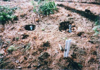
Figure 9: Well and piezometer pair in the foreground, tensiometers in the background.
We monitored the water levels of every well and piezometer at each site everyday through the month of April. The way we measured these levels was by using a stainless steel tape measure with a weight at the end of it. We would lower the weight into a well or a piezometer until it was at a depth such that it was below the water level in the well or piezometer. The length of tape that was in the well or the piezometer was recorded. We then would remove the steel tape from the well or the piezometer and would locate the water mark on the tape. Application of chalk to the tape before lowering it into the well made the water mark easier to see. The difference between the total length of tape in the well and the water mark on the tape gave the depth to water in the well. The elevation of the water table, or the hydraulic head, could then be calculated by subtracting the depth to water from the elevation of the measuring point.
Another aspect to the field study was the installation and monitoring of tensiometers (Figure 10). These instruments measure the soil moisture tension in the unsaturated zone. The tension in the soil, due to cohesive forces of the soil moisture and adhesive forces between the soil moisture and the soil grains pulls fluid out of the tensiometer through the porous ceramic cup at its tip. Since the tensiometer body is sealed, this creates a vacuum with the tensiometer, which can be read from a vacuum gauge or manometer (Figures 9 and 10). As the amount of moisture in the soil changes over time, so does the soil moisture tension, and thus the amount of vacuum within the tensiometer.
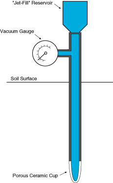
Figure 10: Detail of tensiometer construction.
The tensiometers we used were vacuum-gauge equipped "Jet-Fill" models manufactured by Soilmoisture Equipment Corp. of California. We installed these tensiometers according the manufacturer's instructions, using their coring tube to make a hole for the tensiometer. We then put the ceramic head and O-ring on the base of the tensiometer tube and filled the tensiometer with colored water. Then we allowed enough time for the tensiometer to drip from the ceramic head, to ensure that it was fully saturated. Once this occurred we pumped all the air out of the tensiometer system including the gauge with a hand vacuum pump. When all the air was removed from the system we installed the "Jet-Fill" reservoir head and filled that with colored water as well. This head is used to pump the system after each reading to maintain the vacuum within the tensiometer. The elevations of the tensiometers relative to the wells and piezometers at each site was determined by level surveying at the sites.
One pair of tensiometers was installed at the College Fields site in late September, 1995, and monitored through the month of October. They were removed prior to the ground freezing. Tensiometers were installed at both the College Fields and College Camp sites in March, 1996. Due to the continued threat of freezing in the spring, the tensiometers were filled with windshield washer fluid, rather than colored water, in order to prevent the tensiometer fluid from freezing and cracking the tensiometers. The vacuum gauges on the tensiometers reported the tension in centibars of suction. Hydraulic head values were obtained by unit conversion, and subtraction from the elevations of the tensiometer tips.
We obtained precipitation data covering the duration of our study from the US Army Corps of Engineers at Otter Brook Dam. In addition, we did some of our own snow pack studies, although no interpretation of that data has yet been made. We followed the methods of snow pack and snowfall monitoring discussed by Dingman (1994). To measure snow pack we used a two inch diameter snow tube. The snow tube was plunged into the snow to the ground. The sample of snow in the tube was capped off at the bottom. This sample was measured for total snow volume and then melted to determine actual water content. We also monitored each storm's snow fall by laying a board on top of the existing snowpack and measuring to this board with the snow tube after each new snow fall. Some problems we ran into with these snow pack studies were the lack of constant snow pack, lack of consistent snow falls, and snow drifting.
The results of our infiltration tests are presented in Table 2. In all tests, the initial "instantaneous" infiltration rates are higher than the hour-long rate, which tends to approach the final "instantaneous" infiltration rate. This is consistent with expected behavior, as the initially "dry" soil can more readily accept infiltration. To the extent that the soil under the infiltrometer has become fully saturated during the test, the final rates should approximate the saturated hydraulic conductivity of the soil.
| Site | Date | Initial Rate | Hourly Rate | Final Rate | Soil Moisture Content | Porosity | Degree of Saturation | Soil Survey Estimate |
|---|---|---|---|---|---|---|---|---|
| in/hr | in/hr | in/hr | % | % | % | in/hr | ||
| College Camp | fall | 24.6 | 6.9 | 6.1 | 9.5 | - | - | 6-20 |
| College Camp | spring | 11.2 | 10.2 | 9.8 | 20.2 | 42 | 61 | 6-20 |
| College Field | fall | 20.3 | 14.3 | 11.8 | - | - | - | 0.6-6 |
| Keene Forestry Park | spring | 9.2 | 5.4 | 4.5 | 18.6 | 52.5 | 53.5 | >20 |
Table 2: Results of infiltration tests and soil moisture determinations. The infiltration rates are averages of the results from ten infiltrometers. Soil Survey estimates from Rosenberg, 1989.
Infiltration tests were carried out at the College Camp in both fall and spring, under different soil moisture conditions. The soil was dryer in the fall than in the spring, and thus the initial infiltration rate was much higher in the fall than in the spring. The results from both fall (6.9 in/hr) and spring tests (10.2 in/hr) fall well within the Soil Survey (Rosenberg, 1989) estimate of 6 to 20 inches/hour.
Infiltration tests were conducted at the College Fields site in the fall only. The resulting rates appear to be much higher than the Soil Survey (Rosenberg, 1989) estimate of 0.6 to 6 inches/hour. This might be due to the dry soil conditions in early fall 1995, or to problems with the field methods used in that test.
Results from infiltration tests at the Keene Forestry Park during the spring are also at odds with the Soil Survey (Rosenberg, 1989) estimate of greater than 20 inches/ hr. Our test was performed after several days of precipitation and when the soil moisture content was at 18%. In addition, the condition of the soil surface, in terms of the degree of compaction and the vegetative cover, at the specific site chosen for the test may not have been representative of the soil type.
The soil tension, water table elevation, and piezometric head values from the three sites were converted to common units of hydraulic head, expressed in meters above sea level. Although the relative elevations of the wells and piezometers at each site were determined by level surveying, the elevations above sea level of the sites were determined by map interpolation, so direct comparisons between sites is not recommended. Vertical hydraulic gradients between piezometers, water table wells, and tensiometers (where available) were calculated for each well/piezometer pair. These gradients, as well as the water level data, are presented in hydrographs showing variation over time. In addition, head versus depth profiles have been constructed, as well as cross-sections of each site showing the horizontal configuration of the water table.
The factor that had the greatest impact on the water table level, the piezometric head, and the soil tension was the precipitation in the area. Precipitation data recorded by the US Army Corps. of Engineers at Otter Brook Dam, over the times periods for which we collected water level measurements, are shown in Figures 11a and 11b.
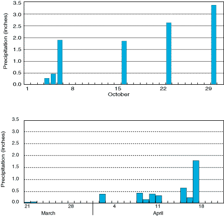
Figures 11a: Fall precipitation, and 11b: Spring precipitation, in inches. Data from the US
Army Corps of Engineers, Otter Brook Dam.
Figure 12 is cross sectional profile of the College Camp site, showing the water table configuration. Notice how the average water levels in the wells are higher then the average water levels in their corresponding piezometers. This indicates that there is a higher hydraulic head at the water table then there is at the base of the well/piezometer pairs. Water always flows from higher hydraulic heads to lower hydraulic heads; therefore the water at this site must be recharging downward into the phreatic zone. The vertical gradients between CC1W & CC1P and the vertical gradients between CC2W & CC2P are shown graphically in Figure 13b. The fact that they are always greater then zero indicates that this site was always recharging over the period of study. This gradient is also apparent in the hydrographs of Figure 13a. Notice how the water levels in CC1W and CC2W are always higher then the water levels in CC1P and CC2P; again indicating downward flow (recharge). The increases in the water levels in the wells are due to precipitation events (Figure 11b). There is a slight lapse in time between precipitation events and the associated rise in water table because it takes time for the precipitation water to infiltrate through the ground to the water table.
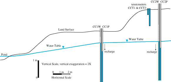
Figure 12: Hydrogeological cross-section, College Camp site
Figure 13c is a hydrograph showing the relationship between the tensiometers at this site (CCT1 & CCT3). Again, increases in the hydraulic heads at the tensiometers can be correlated to precipitation events (Figure 11b). Notice how the hydraulic head of CCT1 rises before the hydraulic head of CCT3--this is because precipitation infiltrating through the soil reaches the 1 foot deep tensiometer before the 3 foot tensiometer. CCT1 also has more variation than CCT3. This may be in part due to differences in soil types: the first foot of soil is mainly loam and the next two feet of soil are more sandy (Figure 3), or may be due to the fact that CCT1 is closer to the surface where the soil may be more readily influenced by changes in atmospheric pressure and moisture conditions.
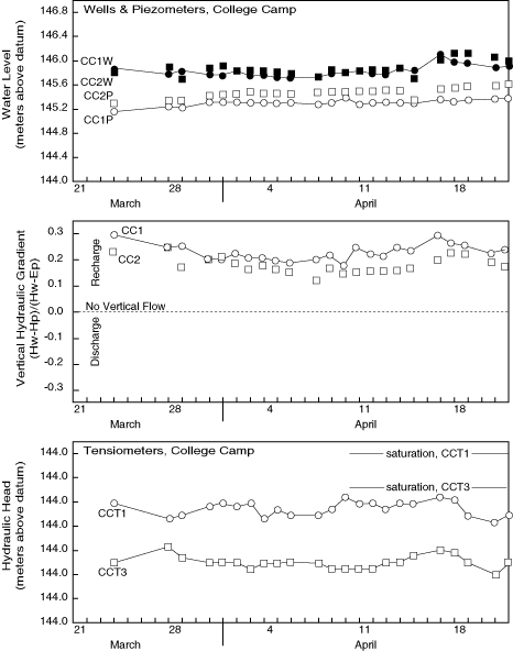
Figures 13a: Well and piezometer hydrographs; 13b: vertical hydraulic gradient; and 13c:
tensiometer hydrographs from the College Camp site.
We monitored the water table and soil tension at the College Fields site in both fall and spring. The general behavior of the hydrologic system was very different in the fall compared to the spring. Figures 14a and 14b show dramatic increases in the the water table elevation at CFW1 and the hydraulic heads at the tensiometers (CFT1 & CFT3). This is due to 2 main factors: 1) the heavy precipitation events towards the end of October (Figure 11a) and 2) the seasonal decline in evapotranspiration as the trees loose their leaves. By late fall, the ground was fully saturated, with localized standing water in low lying spots. This was following a drought condition in the summer of 1995.
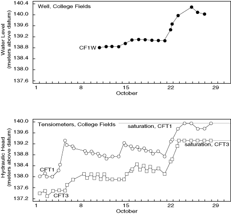
Figure 14a: Well hydrograph; and 14b: tensiometer hydrographs for the College Fields site, for
the month of October.
Figure 15a shows the water levels in CF1W, CF2W and CF2P for the spring; while figure 15c shows the hydraulic heads of tensiometers CFT1 & CFT3. From mid April through much of May, the site was flooded. The hydraulic heads over the spring in this location were, on the average, higher then the hydraulic heads of this site during the fall. This is due to 4 factors: 1) the ground at this site was fully saturated at the end of the fall, and remained essentially so through the winter; 2) heavy snows in late winter and early spring contributed significant spring run-off; 3) periods of relatively heavy precipitation in mid April led to flooding of the area; and 4) trees generally don't bud until late April-early May, so evapotranspiration wasn't a significant factor in removing water from the ground. These factors caused the water table to be high and the soil tensiometers to reach their saturation points in the spring.
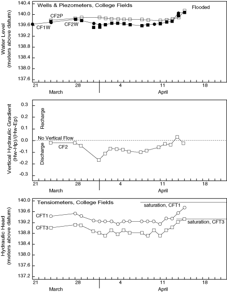
Figures 15a, b & c: Hydrographs from the College Fields site, for the spring.
The water levels of CF1W and CF2W are almost the same throughout the spring. These two wells are located across the College Fields site from one another. This indicates that the water table is essentially flat (in that direction) across the site.
The water levels seem to vary according to the spring precipitation events. Each significant precipitation event yields an increase in water level in both water table wells. In Figure 15a, a significant event occurred between the observations made on April 13th and April 14th. At this point the site changed from a discharge site to a recharge site. Before April 13th, the water level in the piezometer CF2P was higher then the water level in the wells. This indicated that there was a higher hydraulic head at the base of the CF2W & CF2P pair then at the water table; therefore there was discharge occurring at this site. On April 14th, the water level was higher in the water table wells (CF1W, CF2W) than in the piezometer (CF2P). Thus, the hydraulic head was higher at the water table then at the base of the CF2W & CF2P pair. This indicates that the site was recharging on April 14th. This change from discharge to recharge in mid April is shown more clearly in Figure 15b, which shows the vertical hydraulic head gradient versus time. A gradient less than 0 indicates the site is discharging, while a gradient greater than 0 indicates site is recharging.
Figure 16 shows a cross sectional profile of the Keene Forestry Park site, showing the hydraulic gradients at the well/piezometer pairs, as well as the water table configuration. This site contains two wetlands, one in lower section of the site and one in the upper section. The hydraulic gradient determined from the well/piezometer pair KFP1W & KFP1P suggests that the lower wetland may be a "losing" wetland. The hydraulic gradient determined from the well/piezometer pair KFP4W & KFP4P suggests that the upper wetland may be sustained by groundwater discharge from deeper artesian aquifers. Such aquifers do exist in the area, as indicated by the artesian water levels in TW#6 at the nearby College Fields site. The reason why this upper wetland exists is may be due to a local absence of a confining layer below the wetland, which allows the confined aquifer to discharge at this location and create this upper wetland. Well/piezometer pairs KFP2P & KFP2W and KFP3W/KFP3P indicate almost no vertical flow, rather horizontal flow, with minor recharge at the up gradient site, and minor discharge at the downgradient site Figure17a is a hydrograph of the water levels from the KFP wells and piezometers. The constant recharge at KFP1W & KFP1P is very evident by the fact that the water level in KFP1W is always higher then the water level in KFP1P. Likewise the constant discharge of KFP4W/KFP4P is shown by the fact that the water level in KFP4W is always lower then the water level in KFP4P. The lack of vertical flow in KFP2W & KFP2P and KFP3W & KFP3P is show in Figure 17a by the fact that the water levels are almost the same for the well and the piezometer in each pair. This is reinforced in Figure 17b, showing the hydraulic gradients of the four well/piezometer pairs at this site over time.
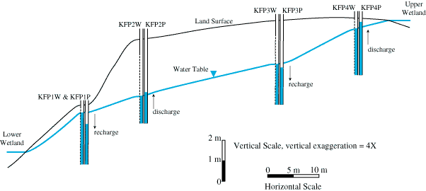
Figure 16: Hydrogeological cross-section, Keene Forestry Park site
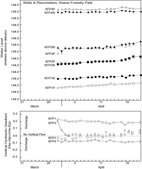
Figures 17a: Well and piezometer hydrographs; and 17b: vertical hydraulic gradients, from the
Keene Forestry Park site, for the spring.
The data we collected in this project shows that the subsurface hydrologic system is dynamic, with significant seasonal and locational variations. We were able to identify downward flow indicating groundwater recharge at the College Camp and Keene Forestry Park sites, at least during the spring when we were monitoring them. These results are consistent with our selection of these sites on the basis of their high infiltration capacities. In addition, our results from the Keene Forestry Park showed significant horizontal groundwater flow from an upper, apparently spring-fed wetland to a lower, apparently "losing" wetland. The subsurface hydrology at the College Fields site was complicated, with the unsaturated (vadose) zone sometimes having a different hydraulic head gradient than the saturated zone. The saturated zone appeared to be dominated by regional discharge from the deep aquifer. In addition, we were able to observe the subsurface hydrologic response to precipitations events at all three sites.
Much work remains, however, in order to more fully understand recharge processes. We did not develop any conceptual model for quantifying groundwater recharge rates beyond the infiltration tests, and only began identifying groundwater recharge areas. An obvious next step is to extend our monitoring over a much longer time period; additional wells might be useful in testing hypotheses about the two wetlands at the Keene Forestry Park site; and an analysis of the lysimeter data from the College Fields might help inform our understanding of the relationship between the hydraulic gradients in the unsaturated and saturated zones there.
This project was supported by a grant from the Keene State College Undergraduate Research Fund to Don Lance and Mike Ravella, and by the Geology Department at Keene State College. The project was conducted as an Independent Study by Ravella and Lance under the direction of Professor Tim Allen, part of on-going work on Ground Water Recharge and the Hydrogeology of Keene. We thank Brian Mattson of the City of Keene for permitting us to install instrumentation at the Keene Forestry Park. We also thank the personnel at the US Army Corps of Engineers' Otter Brook Dam for providing us with precipitation data.
Dingman, S.L., 1994. Physical Hydrology. New York, NY: Macmillan Publishing Co.
Domenico, P.A., and Schwartz, F.W., 1990. Physical and Chemical Hydrogeology. New York, NY. John Wiley and Sons, Inc.
Moore, Richard B., Carole D. Johnson, and Ellen M. Douglas, 1994. Geohydrology and water quality of stratified drift aquifers in the lower Connecticut River basin, southwestern New Hampshire. US Geological Survey, Water Resources Investigations Report 92-4013.
Rosenberg, G.L., 1989. Soil Survey of Cheshire County, New Hampshire. Washington DC: US Department of Agriculture Soil Conservation Service.
Sanders, Laura 1996, Manual of Field Hydrogeology, unpublished manuscript.
Tricker, A.S., 1978. The Infiltration Cylinder: Some Comments On It's Use. Journal of Hydrology., 36:383-391.
Tricker, A.S., 1979. The Design of a Portable Rainfall Simulator Infiltrometer. Journal of Hydrology., 41: 143-147.
Tricker, A.S., 1981. Spatial and Temporal Patterns of Infiltration. Journal of Hydrology., 49:261-277.